Safety stock formula: how to calculate it with AI

‍

Safety stock is the buffer you hold above expected demand to absorb demand and lead-time uncertainty, and the classic safety stock formula sizes it with a service factor, the standard deviation of demand, and the lead time. The number itself takes seconds to compute. The real work is deciding how much risk it should cover and keeping it current as demand and suppliers move.

Watch a planner set safety stock and you will notice the math takes about ten seconds. Pick a method, drop in your demand variance and your lead time, and the spreadsheet gives you a number. Then the real work starts, and it has nothing to do with the arithmetic.

We saw this land in the clearest possible way on a call with a toy retailer’s planning team. One of the planners stopped us mid-demo: she had always assumed the ‘minimum stock’ was simply the figure she typed into the system herself. So why, she asked, was the tool calculating something different underneath? That question is not naive. It is the whole subject. There is the buffer you declare, and the buffer the statistics recommend, and most of the confusion, and most of the cost, lives in the gap between the two.

What the formula actually gives you

Safety stock is the inventory you carry above expected demand to absorb two kinds of uncertainty: demand landing higher or lower than the demand forecast, and suppliers delivering later than promised. Every formula in the textbook is a way of compressing those two uncertainties into a single number.

The quick version, fine when demand and lead times barely move, is max-minus-average:

Safety stock = (max daily usage x max lead time) - (average daily usage x average lead time)

The version most enterprise resource planning (ERP) systems ship adds a service factor and the standard deviation of demand:

Safety stock = Z x sigmaD x square root of lead time

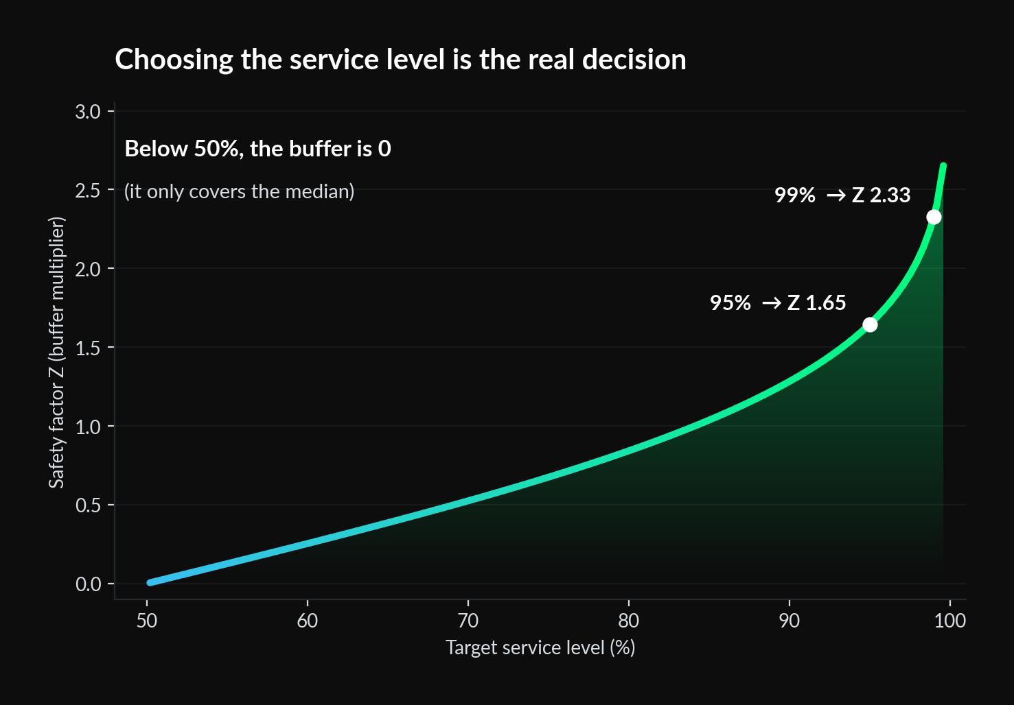
Z is the service factor tied to your target service level (1.65 for 95%, 2.33 for 99%), sigmaD is the standard deviation of demand, and LT is the lead time. When lead time itself wobbles, the formula stretches to cover both sources of variance at once. They all lean on the same assumption: that the variability you measured from history still describes what happens next. That assumption is where the trouble starts.

The decision the textbook skips: which Z

Choosing Z is where the judgment actually happens, and it is easy to get backwards. On that same toy-retailer call, a planner asked whether she could push the confidence setting below 50% to deliberately run a thinner buffer on some lines. The honest answer surprised the room: below 50%, the formula returns a safety stock of zero, because 50% only covers the median forecast. Everything above that line is you buying down risk, point by point.

Almost nobody prices that curve product by product. Teams default to 95% across the whole catalogue because it is the figure everyone remembers from a training deck, not because they have worked out what an extra five points of service costs in cash for that specific item. And a blanket 95% is expensive precisely because it is uniform: a critical spare and a slow accessory get protected at the same cost per unit of risk, even when a stockout on one is a shrug and on the other is a stopped production line. This is also where rule-based methods struggle, and it is worth seeing how DDMRP compares with a probabilistic AI approach.

‍

‍

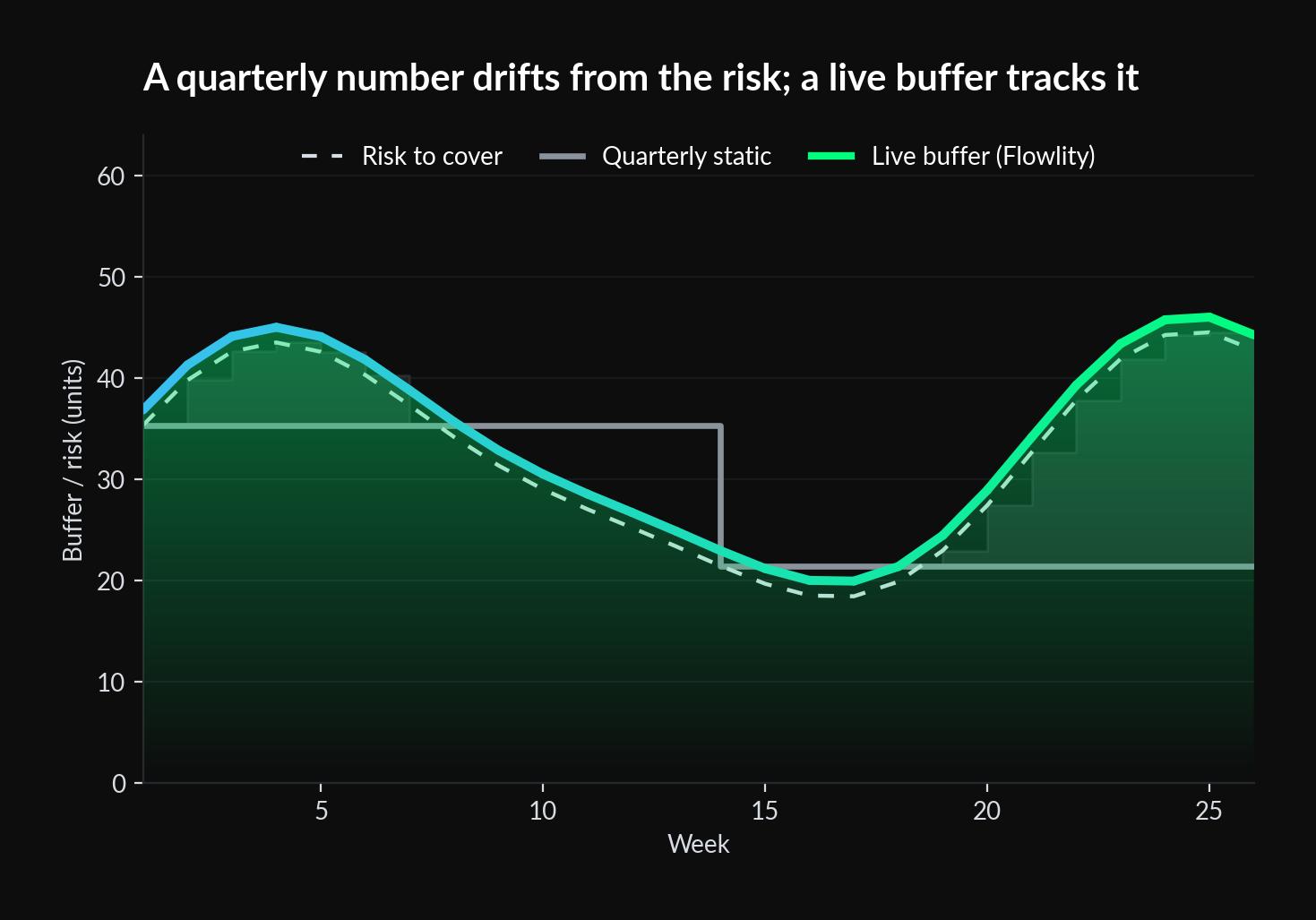
Why a number set once a quarter is already wrong

The formula assumes the variance you fed it is still true when you use it. It usually is not. A planner we spoke with at a footwear distributor put it in plain terms: a month of safety stock is far too much for a product she can restock in two weeks. Except her suppliers, she added, often deliver in three weeks, not two, and allocation makes it messier still. So which is it, two weeks or three? The formula wants one clean lead-time input. Her reality serves up a moving one, and a buffer sized against last quarter’s average is stale by the time it matters.

This is the case for recomputing the number against live demand and supplier performance rather than reviewing it each quarter. Not a marginally better Z-score. A buffer that moves when the risk moves.

The floor on top of the formula

Here is a nuance the calculators skip. Planners routinely set a manual minimum on top of whatever the calculation returns, and they are right to. On the toy-retailer call, the fix was not to override the whole method: it was a lower limit, a floor sitting under the calculated buffer for merchandising or service reasons. If the statistics recommend more, the higher number wins. If they recommend less, the floor holds.

That floor is useful and it is a trap. Applied to a short, deliberate list of references (a strategic account, a single-source component), it is judgment. Layered across the catalogue just to be safe, it quietly rebuilds the same uniform, one-size-fits-all risk tolerance the formula was supposed to replace. The floor should stay the exception, not become the policy.

‍

The formula was built for one product in one place

The classic equation assumes one demand stream feeding one location. Plenty of businesses do not have that luxury. Take a direct-to-consumer accessories brand importing by sea: its planner told us he does not really set a safety stock at all, he hedges lead time, because the honest question is whether the boats take 35 days or 50. Meanwhile he is sitting on far too much stock, not from a bad formula but because the annual budget came in high and the orders were placed against it. No safety stock equation covers that. The buffer was not the problem. The moving inputs feeding it were.

The same blind spot shows up whenever one forecast has to fund more than one channel or warehouse from shared upstream supply. Overcommit to one, the other runs short, and the fix in the moment is an unplanned production run, not a bigger number. That is an allocation problem, and it lives across the network, not inside a single-node formula.

From a static number to a standing decision

The three gaps (stale inputs, uniform risk, single-node math) have one fix. Recompute safety stock continuously against live demand and lead-time data, size it against the business impact of each product rather than a blanket target, and do it across every node the forecast touches instead of one location at a time. That is what AI-driven inventory optimization changes: it turns the calculation into a standing process instead of a quarterly spreadsheet.

The results show up where it counts. A fast-growing direct-to-consumer brand with a wide catalogue replaced rule-based buffers with continuously recalculated, probability-driven ones and cut inventory by 38% without giving up service. The point is not the percentage. It is that a buffer tracking reality week to week behaves nothing like one still running on last quarter’s variance.

A smaller, better-timed buffer also lifts inventory turnover without sacrificing service, because capital cycles through the warehouse instead of sitting against a stale variance estimate.

Treat safety stock as a decision, not a calculation

The formulas are not wrong. They answer how much for one product at one moment and stop, leaving the harder questions (how much risk, how current, how to split a shared buffer) for planners to sort out under time pressure. The teams that get this right stop treating safety stock as a quarterly spreadsheet output and start treating it as a standing decision, recomputed against reality, sized to what each product is worth, and managed as part of a mature, synchronized planning model. The number was always the easy part.

Ready to turn the safety stock formula into a living buffer? Book a demo.