How to optimize inventory without sacrificing service levels

Most inventory optimization techniques assume your world holds still. It doesn't. Demand shifts, lead times stretch, and a reference that behaved like a steady seller in January can read like a new launch by June.

The techniques themselves are sound. The trouble starts when you apply all of them the same way, on a catalogue that never stops moving.

This guide covers the inventory optimization techniques every planner should know, where each one earns its place, and where it quietly fails. Then it looks at what changes when buffers are recalibrated continuously instead of reviewed once a year, and how that single shift lets teams cut inventory without giving up service.

What inventory optimization actually means

Inventory management keeps track of what you hold: counts, locations, movements, reorder points. Inventory optimization asks a harder question. Given uncertain demand, variable lead times and a finite budget, what is the smallest amount of inventory that still protects service? Management is about accuracy. Optimization is about trade-offs.

That distinction matters because it changes the goal. A warehouse can have perfect records and still be badly optimized: cash parked in slow movers, thin cover on the references customers actually ask for. Modern inventory optimization software works the catalogue reference by reference, deciding where a buffer buys real protection and where it only buys storage cost. The output is not a tidier count. It is an inventory profile that frees working capital while holding the service level your customers notice.

Good optimization also respects the fact that not every reference deserves the same attention. A handful of products usually drive most of the revenue, a long tail barely moves, and the interesting decisions sit in the middle, where demand is real but irregular. The techniques below are the standard toolkit for making those decisions.

The eight classic inventory optimization techniques and what they share

The methods that fill most guides have been refined over decades, and each solves a genuine problem. It helps to read them as a set rather than a menu, because they share one assumption worth examining: that the parameters you set today still hold tomorrow.

ABC analysis

ABC analysis sorts references into three classes by their share of revenue or consumption value: a small group of A items that drive most of the value, a larger B group, and a long C tail. The idea is to spend planning effort where it pays, with tight control on A items and a lighter touch on C. It is the most common starting point because it is simple and it forces prioritisation. Its weakness, as we will see, is that the classes are usually set once and left alone.

Economic order quantity (EOQ)

Economic order quantity (EOQ) calculates the order size that minimises the combined cost of ordering and holding inventory. Order too often and you pile up transaction and transport costs. Order too rarely and you carry too much. EOQ finds the balance point for a reference with steady demand and known costs. It works best for stable, predictable items and gets shaky the moment demand or supplier terms move.

Just-in-time (JIT)

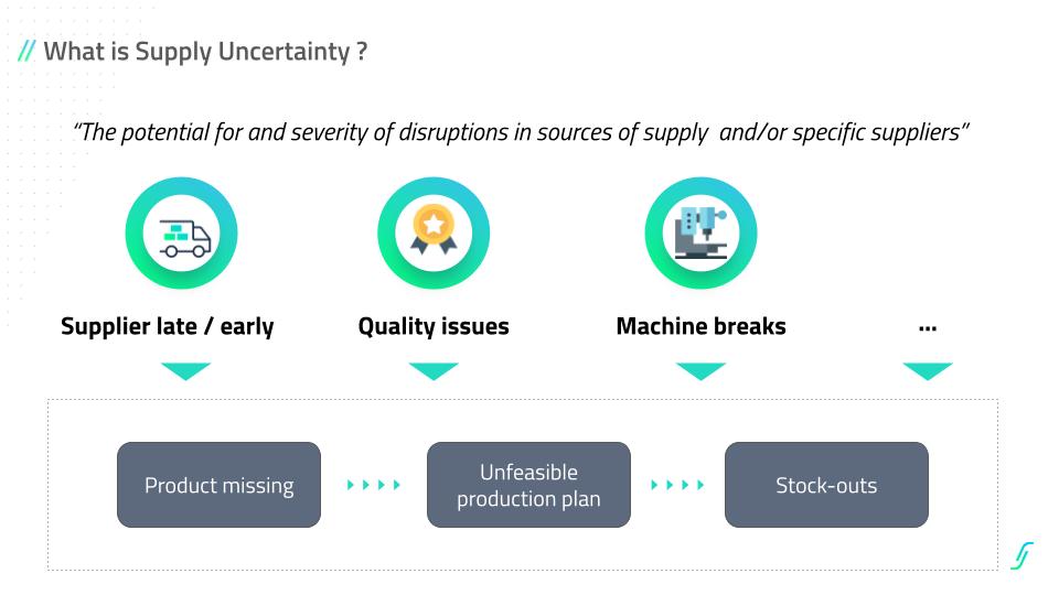
Just-in-time (JIT) aims to receive goods only as they are needed, compressing the inventory you hold to near zero. Done well, it strips out holding cost and exposes quality problems fast. The cost is fragility: JIT assumes reliable suppliers and short, stable lead times, so a single disruption can stop a line. It rewards tightly coupled, mature Supply Chains and punishes volatile ones.

Safety stock

Safety stock is the buffer you hold to absorb the gap between forecast and reality, both demand swings and supply delays. Set it too low and you stock out; too high and you freeze cash. The classic formula ties safety stock to demand variability, lead time and a target service level. The catch is that those inputs are rarely constant, so a buffer sized in spring can be wrong by autumn.

Demand forecasting

Demand forecasting predicts future demand so every other decision, order size, buffer and replenishment, rests on something better than a guess. Traditional approaches extrapolate from history with statistical models. They do well on stable, high-volume items and struggle with intermittent or new references, exactly the ones where a planner most needs help. The quality of your demand planning sets the ceiling on everything downstream.

‍

‍

‍

‍

‍

‍

SKU rationalisation

SKU rationalisation trims the catalogue, retiring stock keeping units (SKUs) that add complexity without adding margin. Fewer references mean cleaner data, fewer buffers to fund, and effective SKU optimization that makes inventory tracking far more accurate. The discipline is deciding what to cut: a low-volume reference can still be strategic for a key account, so the call has to weigh more than unit sales.

Multi-echelon inventory optimization (MEIO)

Multi-echelon inventory optimization (MEIO) optimises inventory across a whole network at once, central warehouses, regional hubs and stores, rather than one location in isolation. It decides where in the chain a buffer protects the most demand for the least cash, which often means holding less locally and more upstream. MEIO is powerful for distributed networks and demanding to run, because it needs a connected view of every node.

‍

‍

‍

‍

‍

‍

Vendor-managed inventory (VMI)

Vendor-managed inventory (VMI) hands replenishment decisions to the supplier, who watches your inventory and tops it up against agreed rules. It can smooth supply and cut the planner's workload, and it works when data flows cleanly and incentives are aligned. It is not a way to outsource the thinking: if the underlying parameters are wrong, VMI just propagates the error faster.

What all eight share is a quiet dependence on stable inputs. ABC classes, EOQ costs, safety stock parameters, forecast baselines, they are calculated from a snapshot and then trusted until the next review. In a catalogue that holds still, that is fine. In one that moves, it is the root of the problem.

‍

‍

The ABC trap: why static classes fail in a volatile catalogue

ABC analysis is usually the first lever a team pulls, and it is also the one that ages worst. The classes are typically set during an annual review and then drive replenishment rules for a year. That is comfortable to manage and dangerous in practice, because a product's behaviour does not wait for the calendar.

Consider what happens across a year. A new reference launches into the C tail because it has no history, then takes off and spends six months underfunded as a C item while demand is really A class. A former hero ages into decline but keeps its A status, so it keeps pulling buffer and cash it no longer earns. Seasonality moves items in and out of relevance every quarter. A class assigned in January describes a catalogue that no longer exists by spring.

The deeper issue is the philosophy underneath. Static ABC treats inventory as something you optimise once in a while, a tidy formula applied on a schedule. Real demand does not run on a schedule. Treating the classification as a fixed truth, rather than a snapshot that needs constant revision, builds a slow but steady mismatch between where inventory sits and where the demand actually is. The method is not wrong. Running it once a year is.

The real trade-off: blind inventory versus intelligent inventory

Most planning debates are framed as inventory versus service. Hold more and you protect availability but tie up cash; hold less and you free cash but risk stockouts. That framing is misleading, because it assumes every unit of inventory does equal work. It doesn't.

The trade-off that actually decides your numbers is blind inventory versus intelligent inventory. Blind inventory is what you place by habit or by a formula that no longer fits: even cover across the catalogue, buffers sized for an average that hides the real variation, safety stock that protects a reference nobody is short of. More blind inventory in the wrong place destroys value without improving the service customers ultimately feel. You can raise inventory and lower availability at the same time, which is exactly the situation that frustrates planners who feel they are holding plenty and still firefighting shortages.

Intelligent inventory is the opposite: every buffer justified by a specific risk and a specific consequence. It concentrates cover where demand is genuinely uncertain and the cost of a stockout is high, and it pulls cover out of references that are stable or low-impact. The total can be smaller and protect service better, because the inventory is doing the job it was placed to do. Seen this way, the goal of optimization is not less inventory or more inventory. It is the right inventory, which is a question of placement and sizing, not volume.

From static formulas to dynamic, probability-weighted buffers

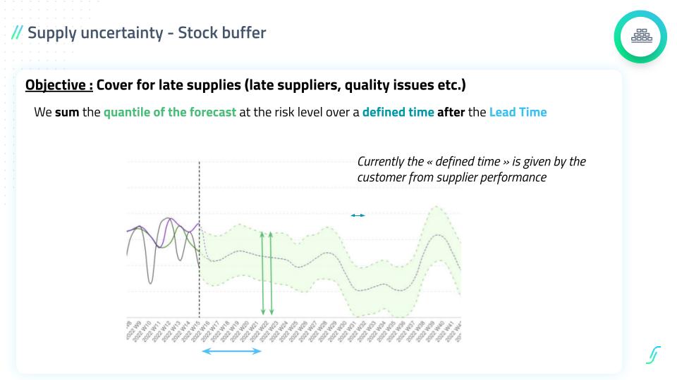
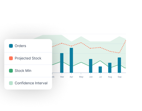
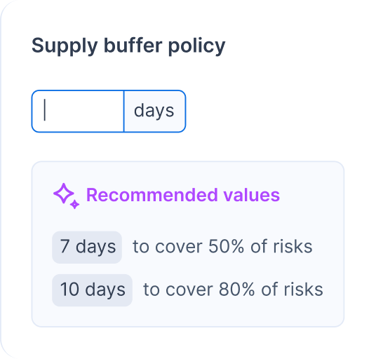
If static classes are the problem, the answer is not a better annual formula. It is to stop treating buffer sizing as a one-off calculation and start treating it as something that recalibrates as conditions change. The cleanest way to express the logic is simple: a buffer should reflect the probability of a risk multiplied by its business impact, recomputed continuously rather than fixed by a class.

Probability of risk captures how likely you are to be caught short on a given reference, which depends on demand variability, lead-time reliability and how much real uncertainty surrounds the forecast. Business impact captures what a stockout would actually cost: lost margin, a damaged key account, a stalled production line. A reference with high probability and high impact earns a generous buffer. One with low probability and low impact earns almost none, regardless of which ABC class it landed in last January. The same reference can move between those states over a quarter, so the calculation has to move with it.

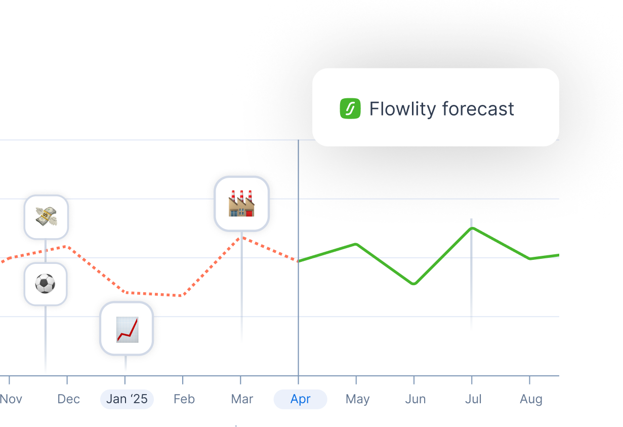
This is where artificial intelligence (AI) changes the work rather than just speeding it up. Machine learning can model demand as a probability range instead of a single number, so the buffer is sized against the actual shape of uncertainty for each reference, not a blanket service-level assumption. It can fold in lead-time variability, seasonality and the recent demand shifts that sensing surfaces, and it can recompute the whole catalogue often enough that the buffers track reality instead of lagging it. The planner stops hand-tuning parameters per reference and starts supervising exceptions: the items where the recommendation and their judgement diverge. That is the practical difference between optimising inventory once in a while and keeping it optimised.

A worked example: cutting inventory without losing service

The theory earns its keep when the numbers move. Across mid-market deployments, teams that shift from static rules to continuously recalibrated buffers typically free somewhere between 20% and 40% of inventory value while holding or improving service, with the range depending on how volatile the catalogue is and how much blind inventory had built up.

Plum Living, a direct-to-consumer interior design brand, is a concrete case. The team carried buffers sized for a catalogue that had outgrown them, with cash spread evenly rather than concentrated where demand was uncertain. The full story is laid out in how Plum Living rebalanced its inventory. By moving to probability-weighted planning that recalibrated cover reference by reference, they cut inventory value from 598,000 euros to 367,000 euros, a 38% reduction, and reached a 21% cut at go-live, all within a three-month deployment. Service held because the inventory that came out was blind inventory, cover on references that did not need it, while the buffers on genuinely uncertain demand stayed protected.

The lesson is not the headline percentage, which depends on the starting point. It is the mechanism. The savings came from re-placing inventory, not from a blanket cut, which is why availability did not suffer. A flat reduction across the catalogue would have hit the wrong references and pushed service down. Targeting blind inventory specifically is what let cash and service improve together.

‍

‍

‍

‍

‍

‍

‍

‍

Inventory cost reduction strategies that survive volatility

Many inventory cost reduction strategies look good in a stable quarter and fall apart in a turbulent one. The ones that last share a trait: they cut cost by improving decisions, not by capping inventory with a blunt rule. A few are worth calling out as options, depending on where your cost actually sits, and several start by digitizing the replenishment process.

The first is segmenting dynamically rather than annually, so cover follows demand instead of lagging it, which is the single biggest lever in a moving catalogue. The second is pooling risk across a network with multi-echelon logic, holding less at the edges and more at a central node where one buffer covers many points of demand. The third is attacking the long tail with honest SKU optimization techniques, retiring references that add tracking complexity and carrying cost without earning margin, which also sharpens the data every other method relies on. None of these is a one-time project. They reduce cost because they keep working as conditions change, which is exactly what a static formula cannot do.

The trap to avoid is the across-the-board inventory cut imposed to hit a working-capital target. It reduces inventory on paper and tends to reduce service in practice, because it takes cover from good and bad buffers alike. Cost reduction that survives volatility is selective by design.

‍

‍

‍

‍

‍

‍

‍

Reading inventory optimization the way a planner should in 2026

The eight classic techniques are not going anywhere, and they should not. ABC, EOQ, safety stock and the rest still describe the real levers of an inventory system. What has changed is the catalogue they run on. Demand is more volatile, lead times less reliable, and product lifecycles shorter than the annual review cycle most of these methods were built around.

That is why the useful question is no longer which technique to pick, but how often to recompute it. A buffer sized by probability of risk multiplied by business impact, and recalibrated as those factors move, turns a static toolkit into a living one. It is also what separates a cut that frees cash and protects service from one that frees cash and quietly erodes it, the distinction at the heart of forecasting and optimizing inventory in a volatile market. The planners who win in 2026 are not the ones holding the least inventory or the most. They are the ones holding the right inventory, and keeping it right as the world refuses to hold still.

‍